For this blog post we are focusing on variable selection for our linear regression model. First we must divide the dataset using the code below.

Now, we construct a model to work backwards to select our variables. Since my dataset has 116 variables I just picked the 8 that made logical sense to include. The output of my code is provided below.

CODE:

fit = lm (dtrn$int_rate ~ dtrn$annual_inc + dtrn$loan_amnt + dtrn$total_pymnt + dtrn$revol_util + dtrn$dti + dtrn$installment + dtrn$total_acc + dtrn$last_pymnt_amnt)

summary(fit)

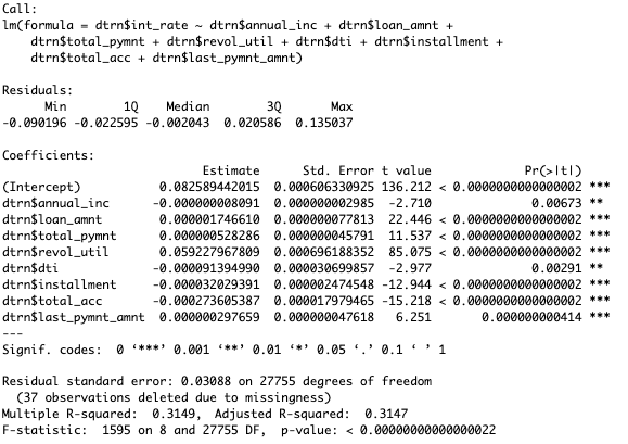
I will only take out the least significant variables for my next round. I can also see in my linear regression model that my R- squared value is .3149, this gives us a baseline.

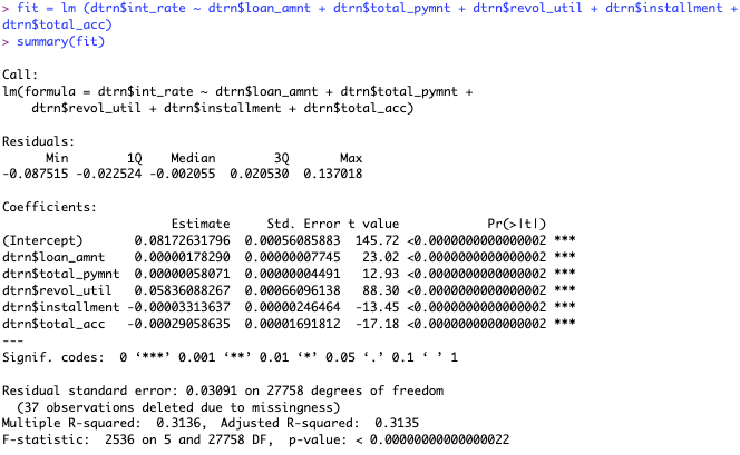
Now all of my variables are significant, but what I didn’t expect was a drop in the R-squared value. The drop is not by much, which most likely helped me because I was overfitting the model. This most likely helped my model be more realistic as I am not using less significant variables. After doing this, I will create my new models with each of the variables in it, creating 16 different models to determine which is the best one. After looking at every single combination, I determined that the one with all of the variables above was the best model based on the R-squared.

In this assignment we have to originally devide the dataset to train R to making a better logistic regression model from our data. I used the code below to do this.

This code made our 2 datasets which we will be using. After this I built my logistic regression model with 2 factors.

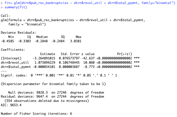
This model is built based off our training data that we divided in R beforehand. All of my predictors are significant, so I will use them in my model equation. The model equation is

log(p/(1-p))= -3.26 + 1.074* revol_until + (-0.000034)* total_pymnt.

(P is the probability of bankruptcy)

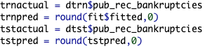
After this now we put in code to make predictions for my test set using the model equation I made. The code is shown below.

After I have created a prediction equation, I will round the probabilities into positive or negative cases for bankruptcy.

Now since all these variables are 1’s and 0’s, I will create these matracies, but this is where I ran into problems. I could not find solutions to the problems online or on Yellowdig, THE END.

Here are the errors I ran into.

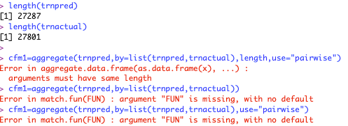
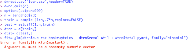
My length could never reach the same size as well, they were off by 80 and I couldn’t find a solution to the problem. I even tried to run the d=na.omit(d) code and it gave me this problem shown below, and also it made the length of trnactual 0.

Thank you for reading.

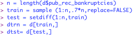
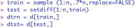
For this assignment, we are told to divide the dataset into training and test sets which we will use to analyze our linear regression model. I used the code below to divide the dataset.

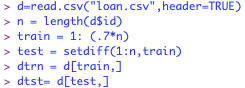
When going about this, I used ID as the length indicator as all loans have a unique ID attached. After this was done, I made n the number of observations within my data, and took about 70% of my data and put it into this training dataset. The test dataset is what is left out of the training dataset, put together in the 4th line of code.

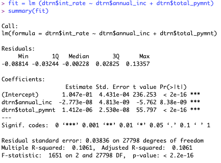
After this, I rebuilt my linear regression model, from blog post 9, within the training data. The data output is shown below, but notice that I changed d$ to dtrn$ to use the training data.

After this, we create predictions for our test data. The code used to do this is shown below.

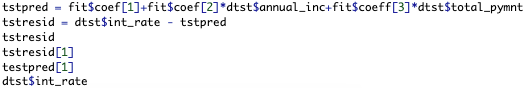
I couldn’t include the data output because it showed too many outputs since I have a large dataset. But after this I needed to create error distributions for my linear regression model.

The plots I used were based off the inputs shown below:

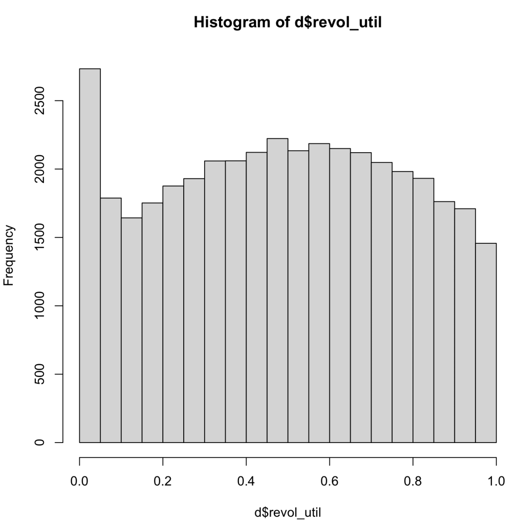
hist(fit$resid)
hist(tstresid)

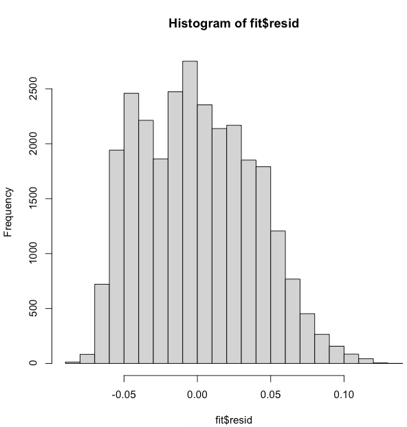
These show a normally distributed graph which is favorable. When I found the mean and medians of the two graphs. When I look at the differences between the data shown below. I came to the conclusion that the means and medians are not close enough to have my linear regression model to be considered stable in the case of the fit$resid graphs.

Above is the same logistic regression model from the last blog post.

log(p/(1-p))= -3.578+ 1.118*revol_util + (-0.00834)*dti

P is the probability of the person having public record of bankruptcies

Multicollinearity Test:

First we have to test to see if our model suffers from multicollinearity. As we can see in the screenshot from R below, our model barely suffers from multicollinearity as the relationship is just over the threshold of 0.25. This means that there is a slight correlation between the 2 predicting factors of revolving credit utility ratio and monthly debt to monthly income ratio, but I am not worried that this will affect my model.

Independent Errors:

I can confidently say that my dataset has independent data-points, because every loan is different and there are probably not many repeat customers within this dataset.

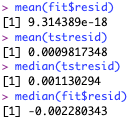
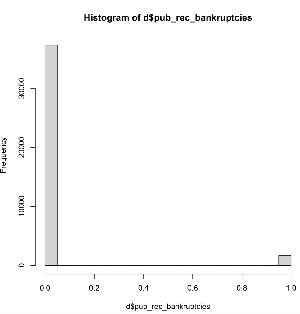
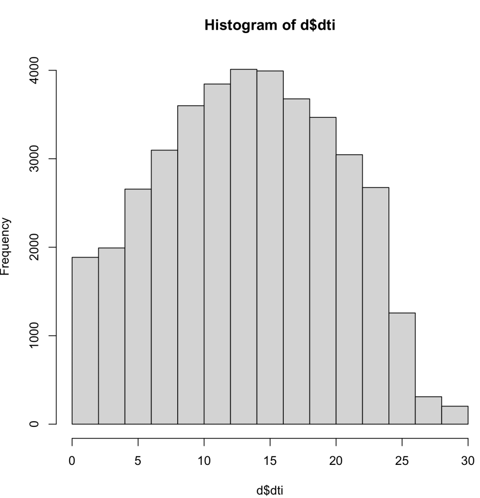
Complete Information:

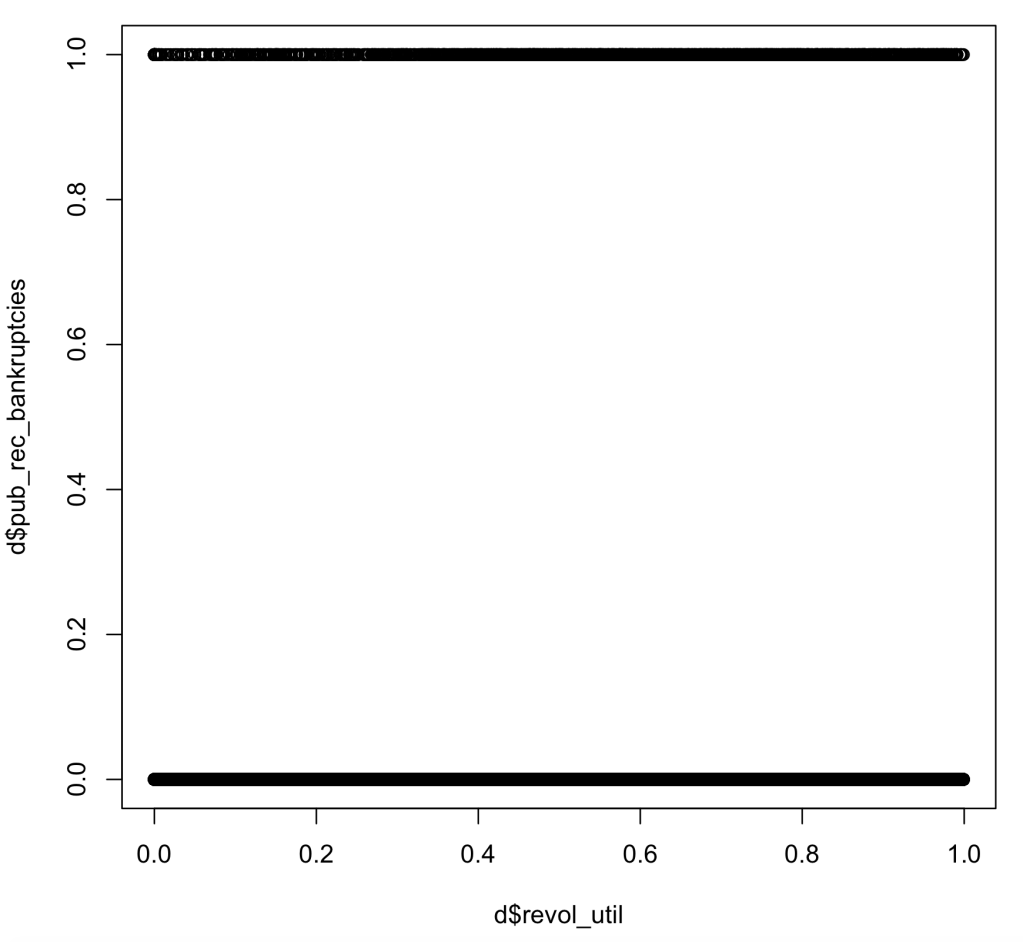
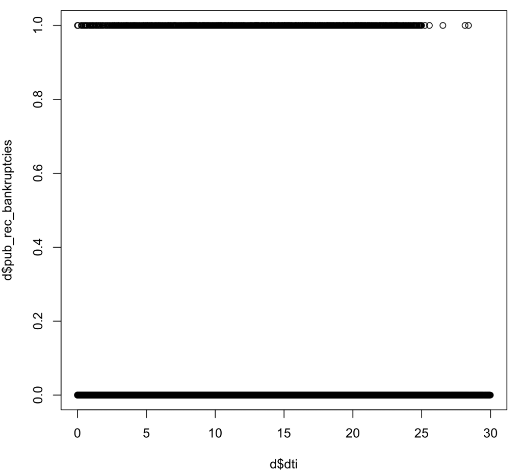
As you can see in the histograms below, we can see that there is a wide range of data for the DTI and the Revol_Util, but there is not as much data diversity within the realm of public record bankruptcies. I did see think this would be a problem with my dataset, because being bankrupt is a fairly uncommon event. Although this is a problem, I do believe that my dataset will have enough variation within the bankruptcies to complete the tasks for this assignment.

Complete Separation:

As we can see in the plots below, we can easily tell by looking at the plot that there is nothing close to complete separation within our data. This is beneficial to my model as it proves that we have large range of data within our binary variable of bankruptcies.

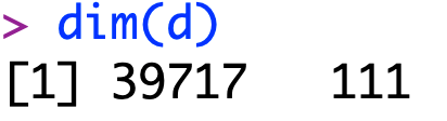
Large Sample Size:

Finally, we will test for a large sample size. As we can tell in the dimensions of my data-set, we do not suffer from this at all as we have close to 40,000 observations, which is plenty of data to work with and draw relationships from.

In conclusion, I believe that my dataset does not fail any of these assumptions as there are logical explanations which do not raise any serious concerns about my data.

For this blog post, we will be making a logistic regression model. For this I will be predicting the binary variable of public record of bankruptcy using borrower’s monthly debt to monthly income ratio. I will also use the revolving line of credit utilization rate to predict this as well.

I used the code in the screenshot below to make this model.

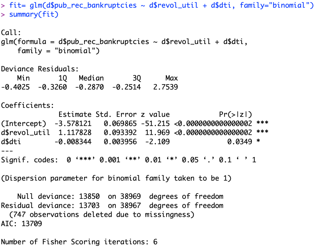
After looking at the logistic regression model, we can tell that both variables are significant in this model as their P-values are close to zero. revolving line of credit utilization rate’s P-value was less than 0.000002 and the P-value for the monthly debt to income ratio was 0.0349, proving significance for both.

After this was done, I plugged my intercept into the model equation and got 0.02717, which means there is a low probability that my model will succeed rather than fail.

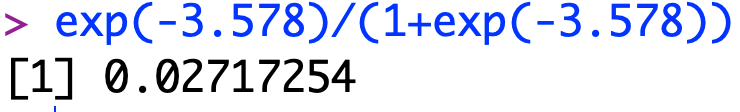
My model equation for this would be log (0.02717/(1-0.02717)). This means that I have a probability of 2.71% for a person to have public records of bankruptcy.

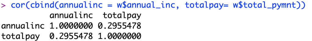
For this blog post I decided to go with my best linear regression model of fit = lm (w$int_rate ~ w$annual_inc + w$total_pymnt).

For this post I will be testing all the assumptions from this module.

Assumption 2:

First, we will test for perfect multicollinearity. As we can see in the screenshot below, we can see that my model does have multicollinearity, but it is far from perfect. We can say this this assumption is true within my model.

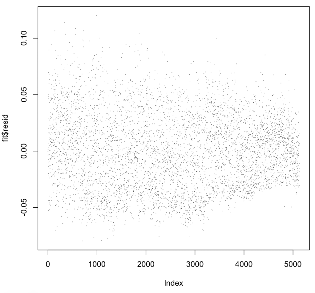
Assumption 3:

Second, we now plot the residual errors of my model. As we can see in the screen shot below, there is no underlying pattern within the plot, so we can say that there is independence within our data, meaning there is no pattern from one datapoint to the next.

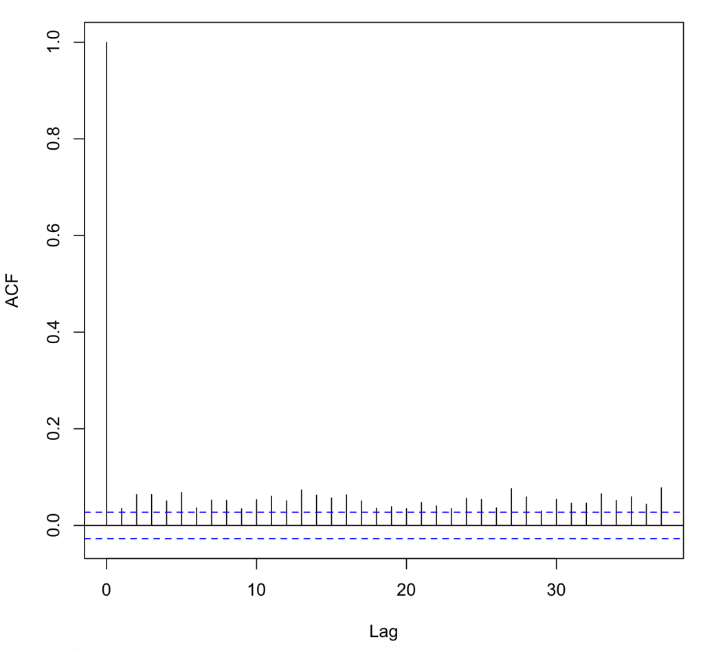
Next, we ran the code acf(fit$resid,pch=20,cex=.05) to see if there is correlation between the errors in my dataset. As we can see below, R says that there is correlation between each of the data points, but this could also be because of a factor like the dataset being sorted in a specific way. I believe this because all of the lags are significant in a positive direction which may likely mean the data is sorted and not random. Unfortunately because of this, my model does not pass this assumption. I will now look at the other assumptions to see if my model is flawed.

Assumption 4:

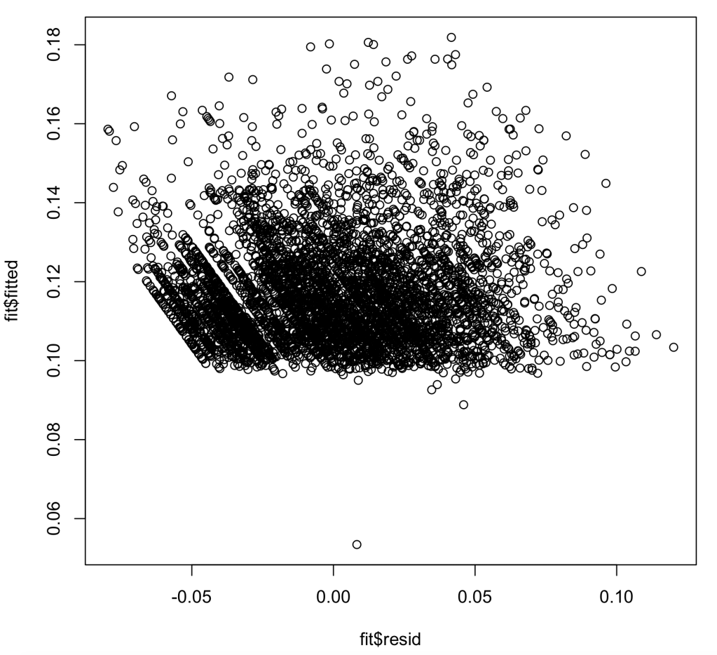
In assumption 4, we are looking to see if my dataset has heteroskedasicity, an unwanted variance in my models ability to predict interest rate within certain ranges. As we can see in the chart below, we pass this test, but we also want to note that most of the values on the chart lie above the Y value of .1. This most likely means that most of my interest rates are above a base rate. We pass this assumption

Assumption 5:

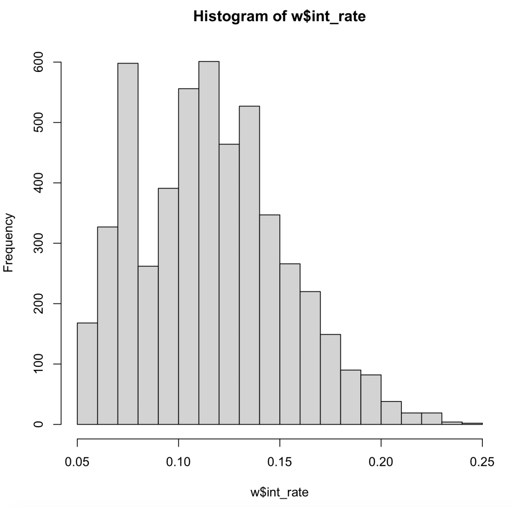
In this assumption we now are looking at normal distribution within our data, as well as our residual errors in our model. First, we look at the histogram of our data. As we can see our data is skewed to the left, meaning the data may not pass the assumption.

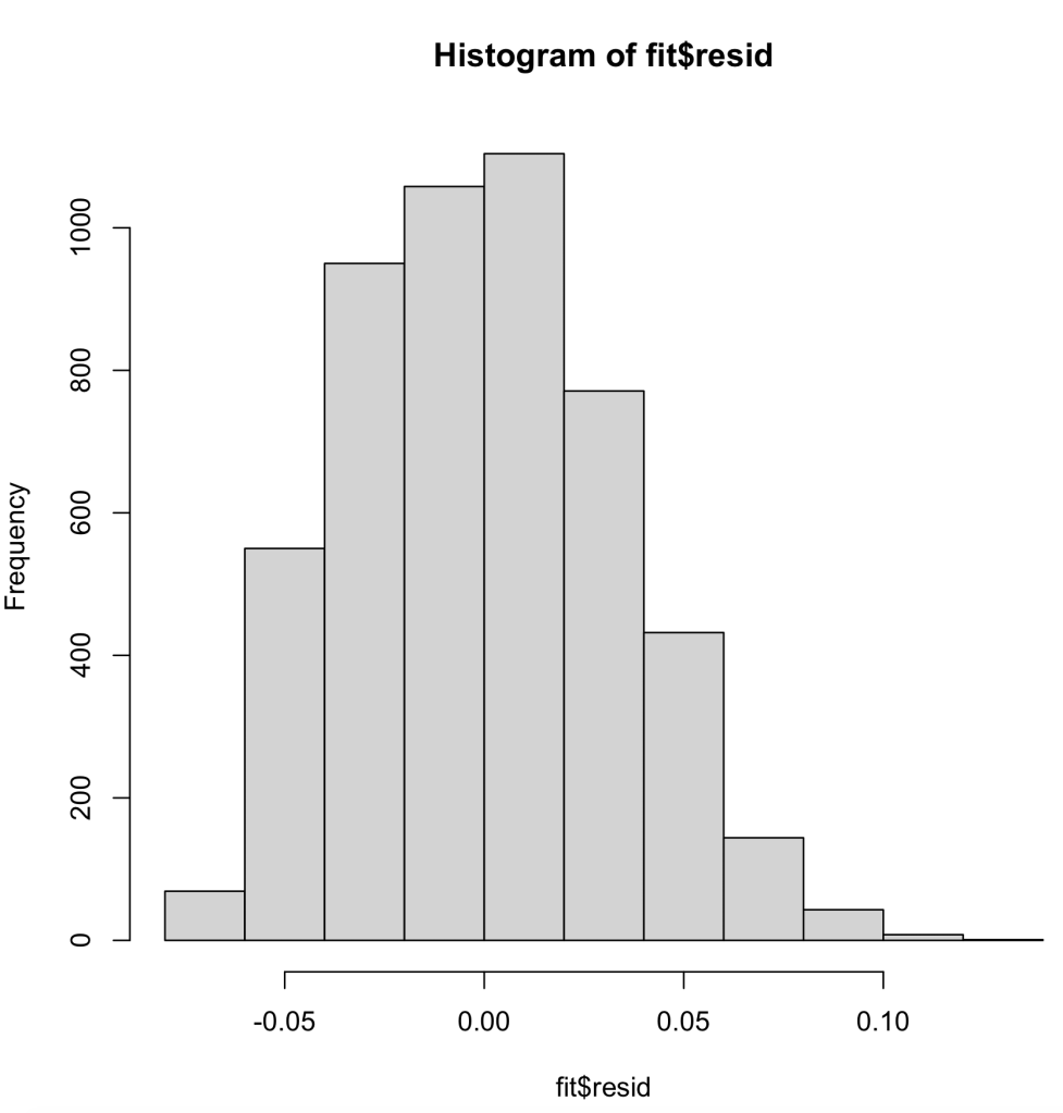
Next, we will look at the histogram of the residual errors within our linear regression model. As we can see here, it is normally distributed, which is a good thing.

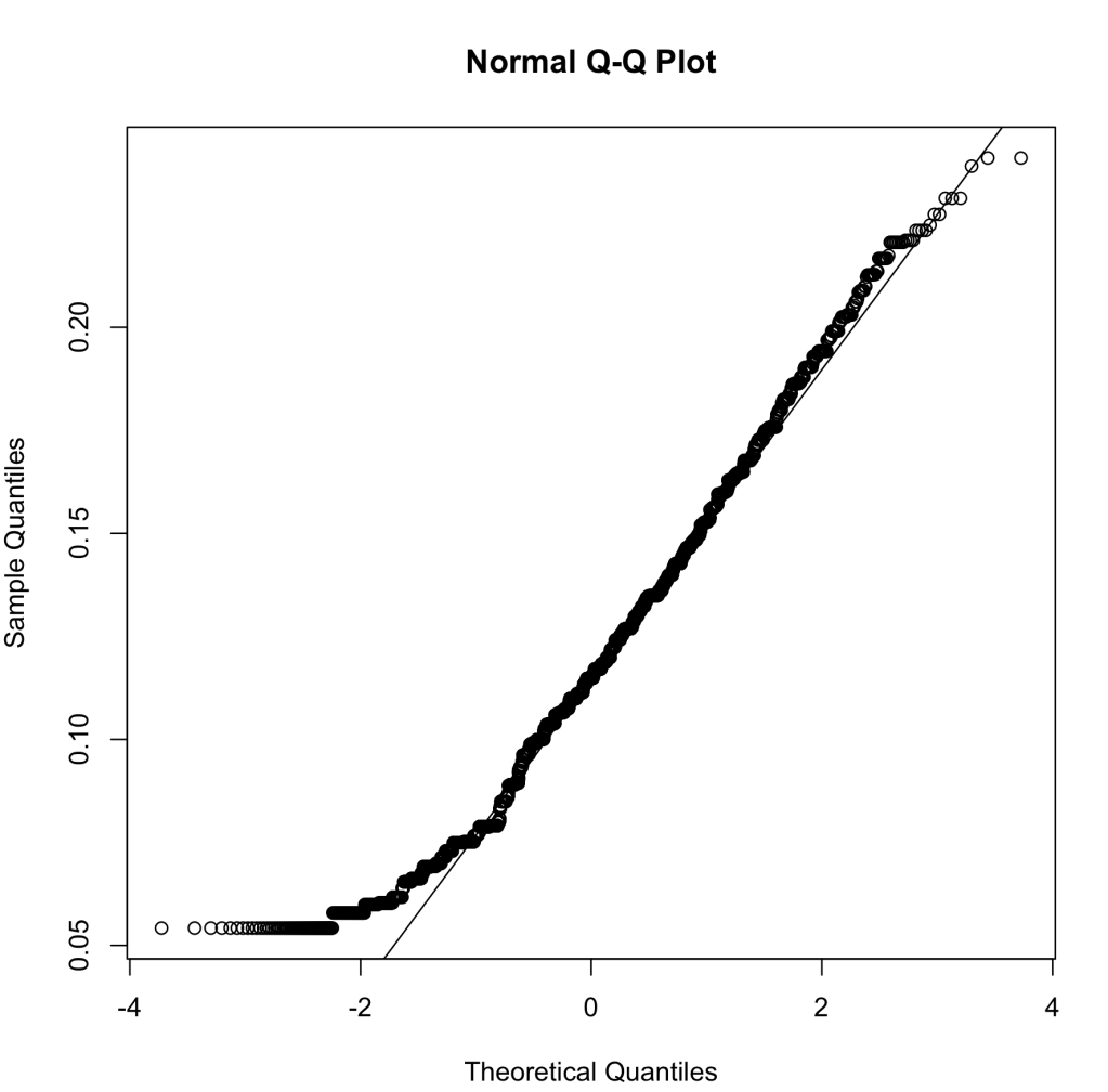
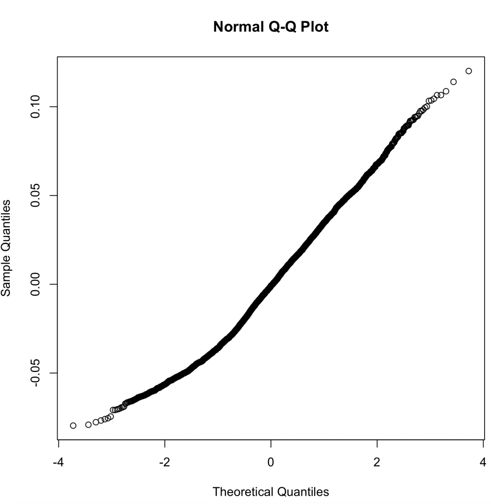
Next to last, we will run the Q-Q plot. This runs the percentiles of the response against the percentiles of a normal distribution. In this plot, we want to see a linear pattern to show that we have a normal distribution. When we run the Q-Q plot for our data, we can see that our data deviates from the line near zero, probably due to the left skewness of our data, but other than that it looks fine.

Finally, we look at the Q-Q plot for our residual errors. This, again, runs the percentiles against a normally distribution for residual errors. As we can see, the trend is fairly linear with deviations in either direction slightly, but to my knowledge this will still pass.

When looking at all my assumptions for my linear regression model, I believe that my model passes every assumption except assumption 3. When we look back at assumption 3, it barely fails the assumption, but it passes every other assumption with only minor hiccups. For this reason, I believe my linear regression model should pass all 5 assumptions due to my explanation of why some of these abnormalities may exist when running these tests of the assumptions.

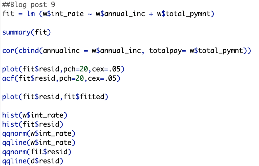
Below are the R codes I ran to get all of these plots:

In my last post for practice, I did a 3 variable model predicting interest rate. The variables I used to predict this were annual income, loan amount, and total payment.

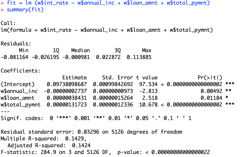
As you can see, all of my variables pass a significance test of an alpha value of .025, so there is significant correlation between my variables and interest rate.

Now we take a look to see if my model suffers from multicollinearity.

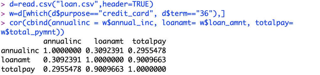
As we can see here, only one pair of my predictors suffers from Multicollinearity. Total pay variable and loan amount varies slightly from each other, but they are almost directly related due to the nature of how loans are eventually paid back in total. The correlation between total pay and loan amount is 0.901. We can tell that there is not much of correlation between total pay and annual income, 0.296. There also seems to be no correlation between the loan amount and annual income, 0.309.

In this blog post, I will be using a loan amount and annual income to predict interest rates of a personal loan for the use of credit card payment. I am now using 2 variables in my linear regression model. I ran this code to better predict the interest rate for a loan compared to the last model discussed in post 6.

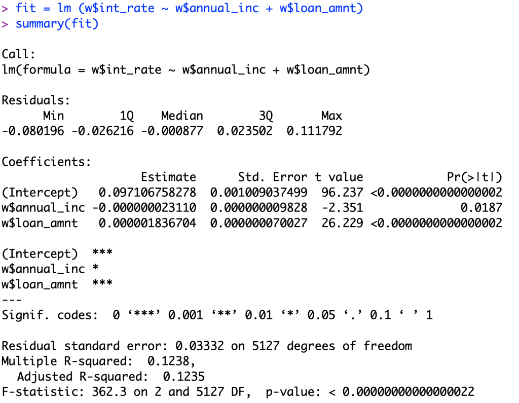
Looking at the p-value, we can see that the even with a alpha value of 0.02, a 95% confidence interval, both our independent variables pass for significance with t values of 26.229 and -2.351. Looking at the second variable, we can see that it is significant, but it is not as good as a relationship compared to our first variable.

In regards to the coefficients, we have a coefficient for annual income of -0.00000002311 which means for every 1 dollar increase in annual income, the interest rate decreases 0.000000023110. To but this in better perspective, for every 10,000 dollars increased it will be a 0.0002311 decrease in the interest rate (0.02311%). Now, looking at the loan amount coefficient we can interpret this number as for every 1 dollar increase in the loan, we will normally see a 0.000001836704 increase in the interest rate. Again to put this into perspective, for every 10000 dollars increase in the loan, you will see an increase in the interest rate of 0.01836704 (1.837%).

When we look at the R-squared value of 0.1238, we can interpret this as 12.38% of the data variation is described by the relationship between the 2 variables tested within our linear regression model. On the other side of this number, we can see that a whopping 87.62% of the data variation is NOT explained by the 2 variables, which leads me to believe that there is some other factor that may be affecting interest rates outside of the dataset. Between this linear regression model and the one shown in post 6, there has been a .07 increase in the R-squared value. This leads me to believe that there is not a huge difference when adding the second variable into the linear regression model, even though the second variable IS significant to interest rates.

Just for fun, we will see what happens if I add a third variable into the set.

Something that I noticed when I added this third value of total payment is that the R-squared value increased, BUT also decreased the significance of the annual income and loan amount when determining a relationship between the variable and interest rates.

Plot twist! I changed my data set yet again!

Due to the fact the last dataset was not useable due to corruption of an entire economy, funny how that stuff just “happens”. Now, we are focusing on personal loan rates with data from the lending club. We will try to determine what an interest rate for a person who is applying for a personal loan would be. We will just be looking at loans to pay off credit card debt to try to find commonalities from loan to loan. The variable I will be using to predict this is loan amount.

BUT, for this blog post I will be explaining the relationship of my R-squared value of my new linear function. So, first I will show you my new relationship for this dataset.

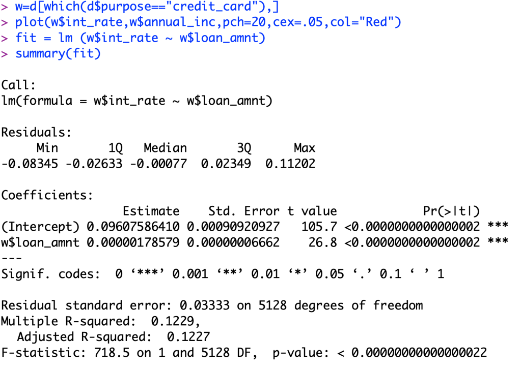
Now, we see that this is a significant relationship because our p-value is close to zero. Now that we got that out of the way we now will look at our R-squared value. Our value for this is 0.1229. What this means is that for all of our data, 12.29% of its variation is able to be explained by this relationship. That means that 87.71% of the data variability in the interest rates are not explained by the loan amount. Now, this a low R-squared value, but out of all of the continuous variables given in the dataset, this is the best model to predict this continuous variable.

In this post I will be comparing 2 different predictive variables to find out which variable is better at predicting the variable in question. These variable we are trying to predict in this dataset is Net Value Growth Rate. We are using Cash Reinvestment % and Cash Flow per Share to predict this growth rate of the companies. We are comparing the 2 predictive variables to find out which one is better at predicting this growth rate.

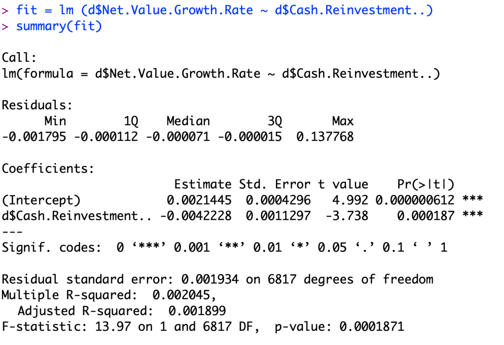
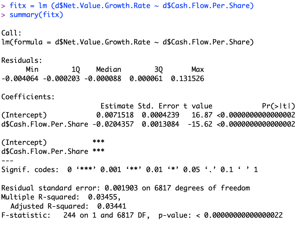
After looking at the data, you can see that the Cash Flow per Share ratio is a better indicator to what a company’s growth rate is going to be. You can tell that the linear regression model in the second picture is going to be a better predictor than the first picture because when you examine the p value for each linear regression model, you notice that the second one has a value near zero. The equation of my new linear regression model is Y=0.0071518+(-0.0204357)X since it fits better than the previous linear regression.

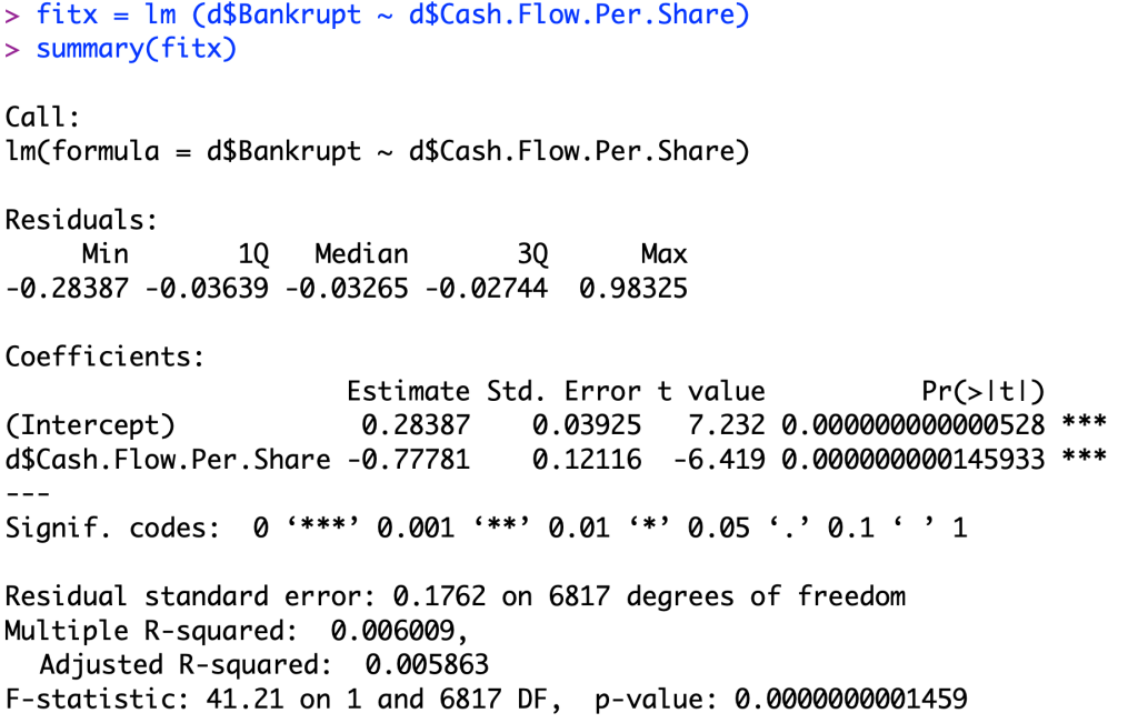
The equation for this linear regression model is Y=0.28387+(-0.77781)X.

To understand this model, we will first look at the intercept. This intercept of 0.28387 and a t-value of 7.232, rejecting the null hypothesis of the intercept being equal to zero, because it is more than 2.95 standard deviations away in the t-distribution. This value means that for businesses that are still alive, they have on average a cash flow per share ratio of 0.28387. And for the coefficient, this value means when the company goes out of business, on average it has an average cash flow per share that is 0.77781 below the average living company (0.28387).